How to Use VLOOKUP in Google Sheets (Step-by-Step)

If you regularly play with large data sets or create dynamic reports and dashboards that need to find specific data against different values, you’ll love the VLOOKUP function in Google Sheets.

VLOOKUP or Vertical Lookup is an advanced function in Google Sheets that can scan thousands of cells vertically, find the relationship between different sets of values, and display the data that you are searching for in the cells you want.

Sounds confusing? Don’t worry.

By the end of this article, you’ll know exactly what is VLOOKUP and how to use it in Google Sheets to save time and create dynamic reports for any data sets.

Let’s dive in.

What Is VLOOKUP In Google Sheets?

VLOOKUP or Vertical Lookup is a function in Google Sheets that allows you to search vertically from top to bottom for a value (search_key) in a table (data range) and return the value of a specified cell in the row of that value (search_key).

The results of the VLOOKUP function are dynamic which means they’ll change when the values of the cells used in the formula change.

Let me simplify this with an example.

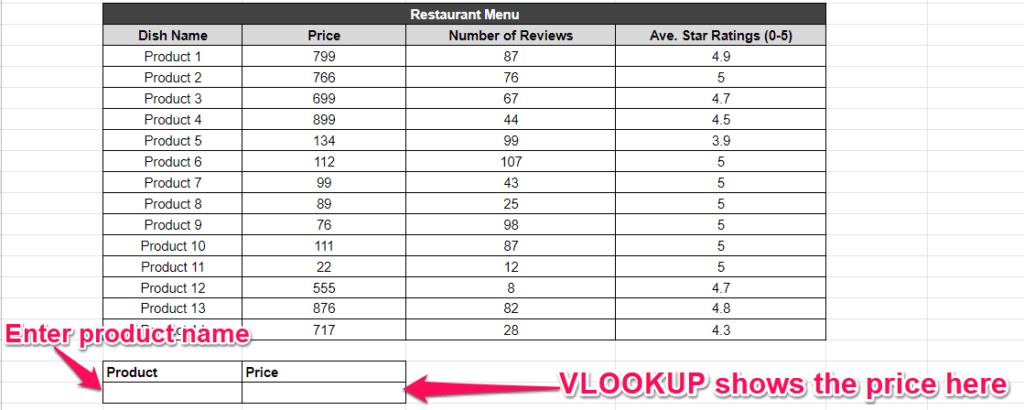
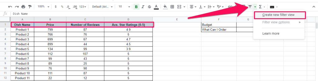
Imagine a restaurant menu that lists soups, salads, starters, main course dishes, and desserts along with their prices, number of reviews, and the average star ratings.

With the VLOOKUP function, you can set up a cell in which you’ll enter the name of any dish from the menu and VLOOKUP will show you the price listed next to it in the menu.

Got it?

You can also use VLOOKUP to find the cheapest item on the menu, the one with the most reviews, the best star ratings, or the items within a certain price budget.

That’s like scratching the surface of what VLOOKUP can do for you but I’m sure this would’ve made it clear what the function does for you.

Later in the article, I’ll share multiple examples of how you can use VLOOKUP to make its utility even clearer.

Why use VLOOKUP?

I don’t know about you but I don’t like the idea of manually searching hundreds of values in a spreadsheet or table and entering it in another cell.

And even if someone loves doing this manually, they’ll need to update those values every time the original value changes.

VLOOKUP not only does this automatically in less than a second but also allows you to play with your data in several different ways.

For example, you can pull data from different sheets, set criteria to filter out values from your results, and always get the latest updated results based on your original data.

Plus, since all the data is coming automatically without any human interference, the chances of any errors in your results are next to zero.

Your only job is to ensure that your tables or spreadsheets have the right data and the VLOOKUP function is using the right criteria.

Google Sheets will take care of the rest.

VLOOKUP vs. Find (Ctrl+F) – What’s the Difference?

CTRL+F is a popular keyboard shortcut you can use to find any value in Google Sheets (and most other document management programs).

But is it similar to VLOOKUP?

Not even close.

CTRL+F is a keyboard shortcut, not a dynamic function in Google Sheets.

You can use it to manually find values in a sheet but you can’t use it in a cell to automatically find data.

VLOOKUP, on the other hand, is a cell function that pulls in dynamic results based on your original data source.

Plus, it can match different data sets, filter out results that don’t meet your criteria and display its results in the cells you want.

In short, there’s no similarity between CTRL+F and VLOOKUP.

VLOOKUP Syntax In Google Sheets

Here’s the standard VLOOKUP formula in Google Sheets

Let me explain each component of this formula separately.

For better understanding, let’s use the same table I used earlier in the article.

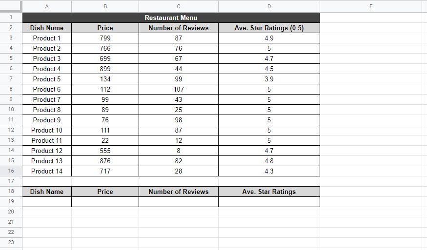
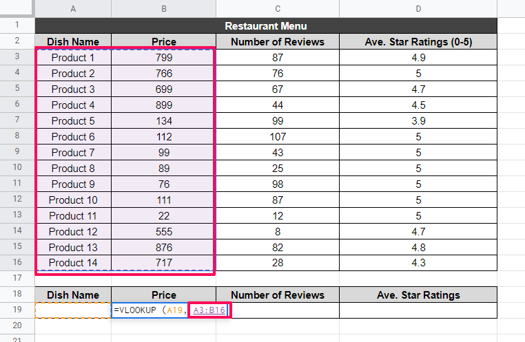
Search_Key: This is the cell that contains the value that you want to search for in a given data set. It is also called a lookup value or unique identifier. If we take the example of a restaurant menu, search_key will be the names of the dishes/products on the menu for which you want to search the price. In this example, you’ll enter that value in cell number A19.

Range: This is the data range that you want to consider for the search. The first column of the range is used for searching the value in search_key. For example, if we select the first two columns of this table (Dish Name and Price) our range will be from cell A2 till B16 while the first column (Dishes) will be used for searching the value you enter search_key.

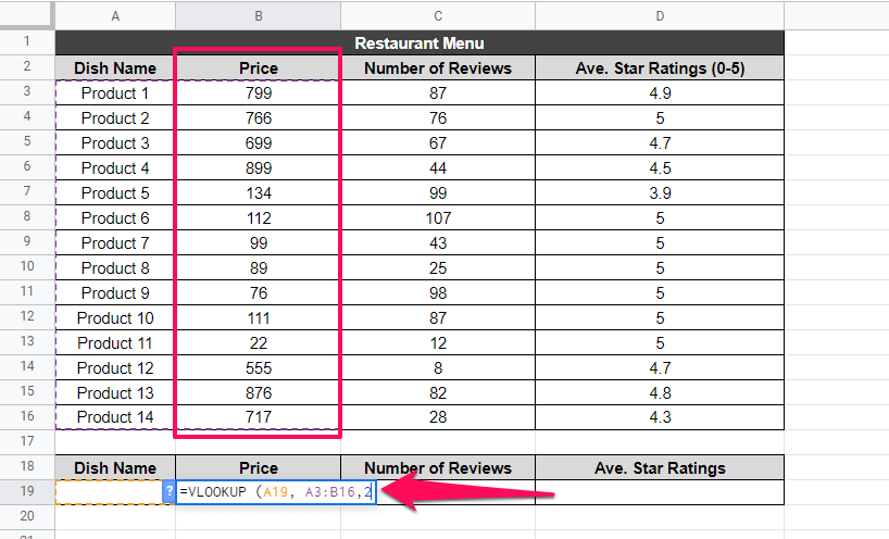
Index: This is the column in which you want to search the corresponding value for search_key. In the formula, you’ll represent this column by its serial number relative to the first column in your data range. For example, if your data range is A2:B16, your search_key value is A19, and you want to find the Number of Reviews for Product 3, the index number for this column will be 3 in your formula (the first column of the range, Dishes, is always denoted by 1).

[is_sorted]: This represents whether the data in the column you want to search (the first column from the left) is sorted or not. If the data is sorted, you’ll type TRUE. If it’s not sorted, you’ll type FALSE. If you leave this part blank, it’ll be set to TRUE by default.

What are the implications of this option?

FALSE: If you set this part to FALSE, the formula will return an exact match result of the value you’re searching for. In case multiple values meet your search criteria, the first one will be shown. And if no value matches your search, the function will show #N/A.

TRUE: If you set this part to TRUE, the formula will return a value that’s less than or equal to your search key (whatever is the closest). If all values in the search column are greater than your search key, it’ll show #N/A.

To sum up this section, here’s how you’ll use VLOOKUP to search for a product’s price on the menu

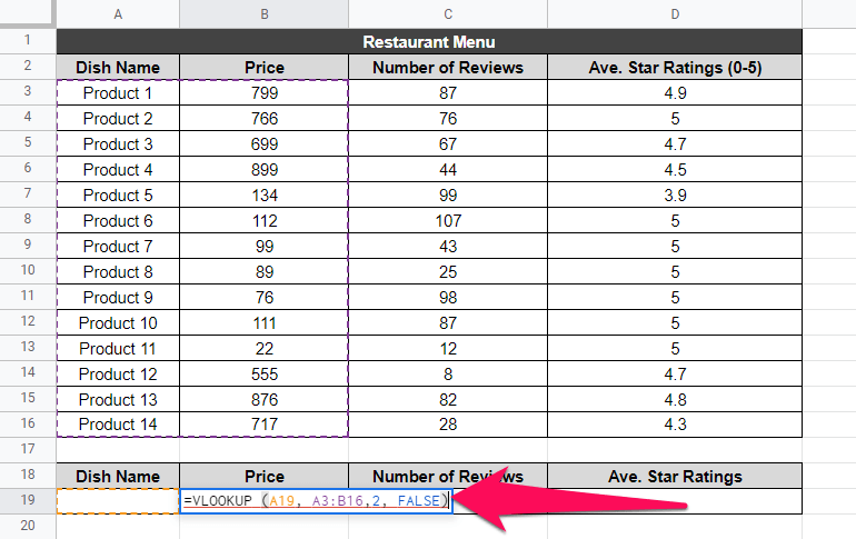
Here’s how the syntax appears in Google Sheets

You can apply this function to multiple cells in a sheet to show different results or search multiple values within a data set.

How to Use VLOOKUP in Google Sheets For Exact Match Searches

Using VLOOKUP in Google Sheets is pretty simple as I’ve shown you in the previous section. But let me share the step by step details of the process so that there’s no confusion left.

Step 1: Open Google Sheets on your computer
Step 2: Open the file that contains the data set that you want to search.
Step 3: Click on a cell outside your data set where you want to display your search results.

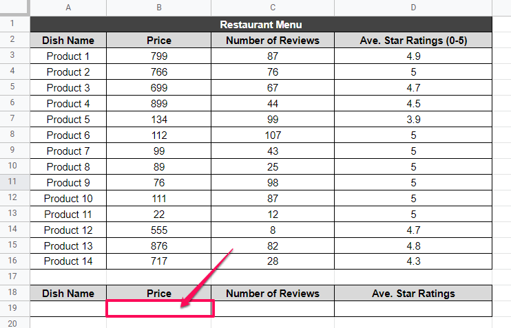
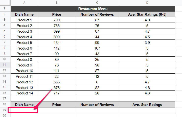
Step 4: Now determine the cell where you will enter your search key.

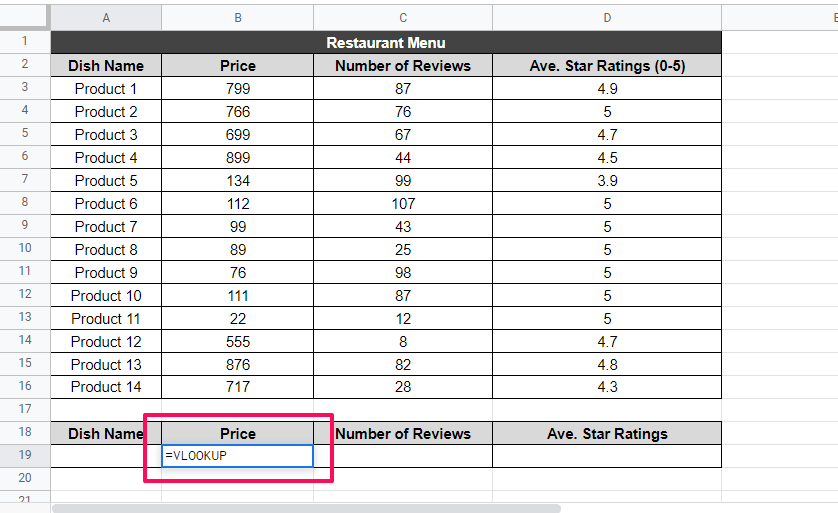
Step 5: Apply the VLOOKUP function to the relevant cell.

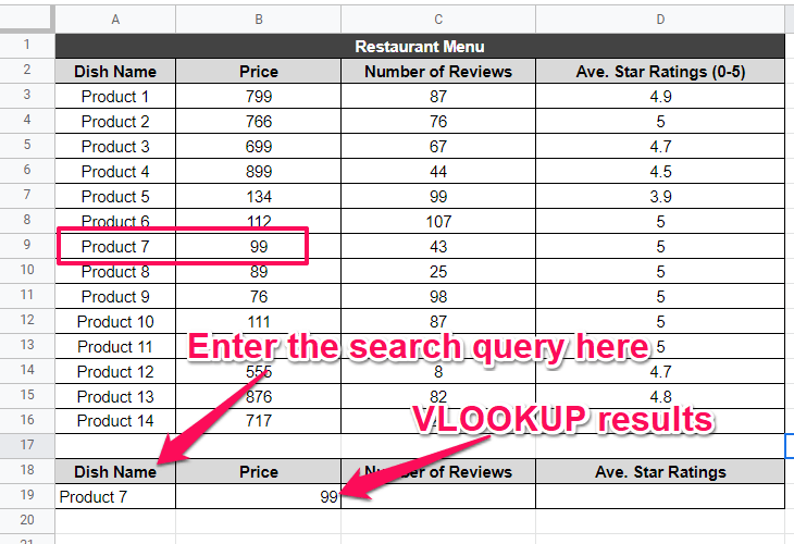
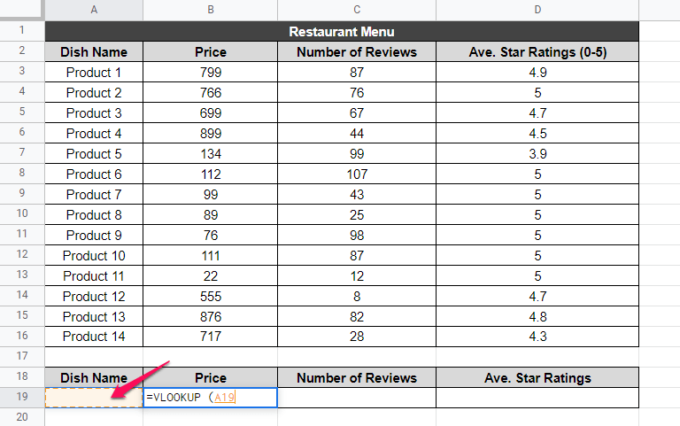
Step 6: Choose the cell where you’ll enter your search key. In this example, it’s A19.

Step 7: Choose the data range where you want to search for your search key. In this example, the data range is from cell A3 to B16.

Step 8: Now choose the column from where you want to pull the corresponding value for your search key. In this example, the column is Price which means we’ll denote it by 2 since it is the second column in your data range.

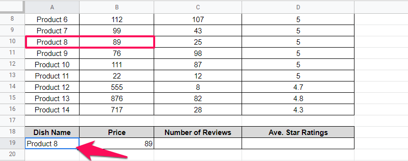
Step 9: We want to find the exact price of the product name we enter therefore we’ll set the [is_sorted] parameter as “FALSE”.

Step 10: Press the ENTER key to complete the VLOOKUP formula in your Google Sheets cell.
Step 11: Now enter the product name in the search key cell to find its price.

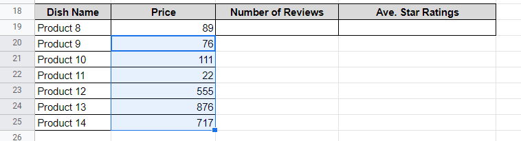
Step 11: If you want to apply this formula to the cells below it, simply select and drag it down till the cell you want. Do this for both the search key cell and the cell containing the VLOOKUP formula.

How to Use VLOOKUP in Google Sheets For Closest Match Searches

If you want to find the closest match to your search key instead of an exact match search, you’ll set the [is_sorted] parameter to TRUE.

In the restaurant menu example, let’s say you want to find the product that’s closest to your budget.

Here’s how you’ll use VLOOKUP to find it.
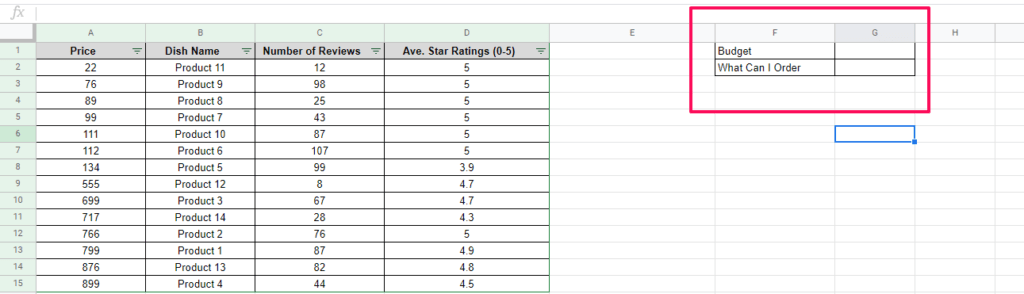
Step 1: First of all, sort your data in a way that the price column comes before the product list because VLOOKUP cannot search on the left of your data-range.

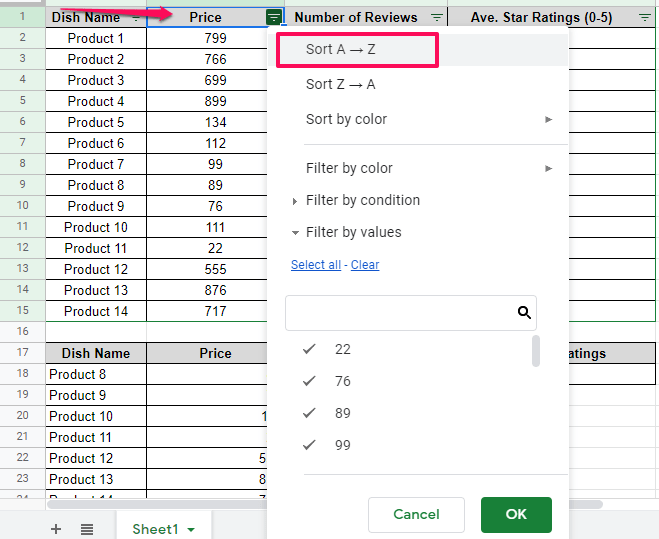
Step 2: Now apply filters on your data set.

Step 3: Sort the price column from A to Z (ascending). If the data is not sorted in ascending order, the VLOOKUP function for variable match won’t work properly.

Step 4: Now create two separate cells outside your data range. One for entering the search key and the other to display the results of VLOOKUP.

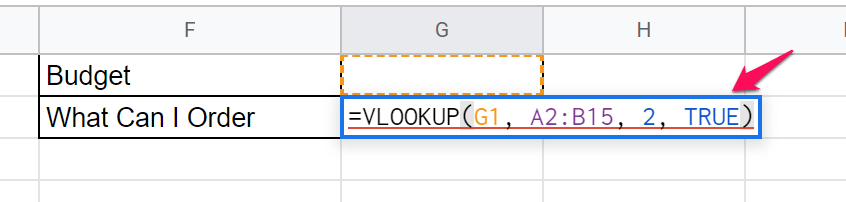
Step 5: Now apply the VLOOKUP function the same way as described in the last section.

Step 6: But this time set the [is_sorted] parameter to TRUE instead of FALSE.

Step 7: Now enter your budget in the search key cell.

Step 8: VLOOKUP will show you the product name that’s equal to or less than your budget (closest match).

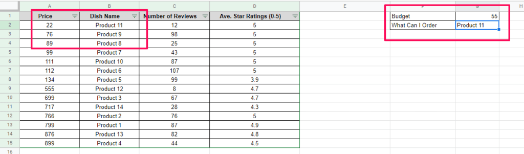
As you can see, the budget I entered is 55 for which VLOOKUP shows Product 11 as the only item in my budget.

If you look at the table on the left, there’s no item with a price tag of 55. So the next closest match is Product 11 with a price of 55. The rest of the items are priced higher than 55 and as I mentioned earlier, VLOOKUP only searches for values that are equal to or less than your search key.

In these examples, we applied VLOOKUP for data in a single Google Sheet.

Let’s see how to use VLOOKUP for multiple Google Sheets.

Using VLOOKUP In Multiple Google Sheets

You can use VLOOKUP to pull data from multiple Google Sheets as well.

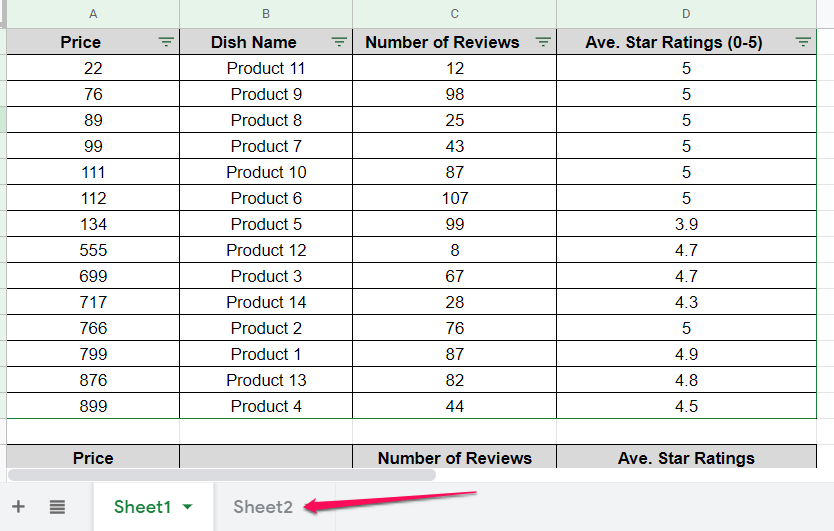
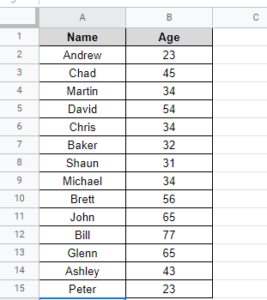
Suppose we have another sheet (Sheet 2) in our file that contains the names and ages of our customers.

If you want to pull the age of the customers in Sheet 1 by entering the customer’s name, here’s the formula we’ll use.

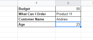
Step 1: Create the cells where you want to enter the customer name (search key) and pull their ages from the other sheet.

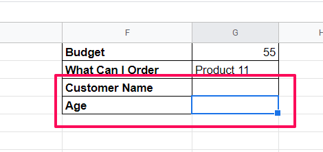
Step 2: Enter the VLOOKUP function to the age cell.

Step 3: Choose the cell next Customer Name as your search key.

Step 3: When choosing the data-range, click on Sheet 2 and select the two columns in the data range.

Step 4: Press enter to complete the function.

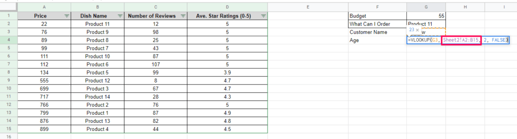
Step 5: Now enter the customer name in the search key cell to pull their ages from Sheet 2.

Using the same format, you can pull data from as many sheets in a file as you want.

Can You Confidently Use VLOOKUP In Google Sheets?

I’ve shared the basic syntax and some of the common uses of the VLOOKUP function in Google Sheets. As you can see, it’s a handy function that can help you search through thousands of cells and find the information you’re looking for. The examples I’ve shared in this article are very basic so that you can understand how this function works. But there are many advanced ways you can use it as well. So go ahead and experiment with large data sts using the VLOOKUP function to see how it can make your work easier. Let me know if you have any questions.