The 12 Excel Shortcuts You’ll Regret Not Using Sooner

If you’re a frequent user of Microsoft Excel, you can add several months to your life by using Excel shortcuts.

I’m not joking.

According to a study, you can save 64 hours every year by using keyboard shortcuts as a frequent Excel user.

There’s so much you can do with Microsoft Excel and using the right keyboard shortcuts at the right time makes it more enjoyable (plus helps you make an impression on your bosses)

In this article, I’ll share some of the most useful Excel keyboard shortcuts and how you can use them to get things done faster.

Let’s get started.

Shortcut #1: Insert A Note/Comment On A Cell

If you’re working on an Excel sheet that you have to share with your team members or just want to add reminders to a cell for your reference, you’ll love this keyboard shortcut.

It allows you to add comments to a cell that users can view by hovering over it.

To use it, click on the desired cell and press SHIFT+F2 on your keyboard. This opens a comment box where you can leave additional notes, reminders, or any other information that provides context to the cell’s value.

Here’s how it appears in Excel.

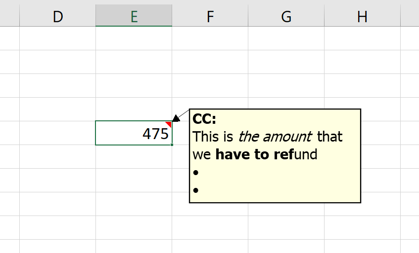
The great thing about the comment box is that you can also add bullets and formatting to it like a normal cell.

The cells with a comment box have a small red mark for identification.

Shortcut #2: Toggle Auto Filter In Columns

If you’re used to playing with heavy Excel worksheets that have lots of data, you’ll find auto filter a real lifesaver.

Applying filters to a cell allows you to extract the information you’re looking for, organize the data in different ways, and identify trends within data sets.

The keyboard shortcut for applying filters in MS Excel is simple. Press CTRL+SHIFT+L after selecting the first cell of the column where you want to apply a filter.

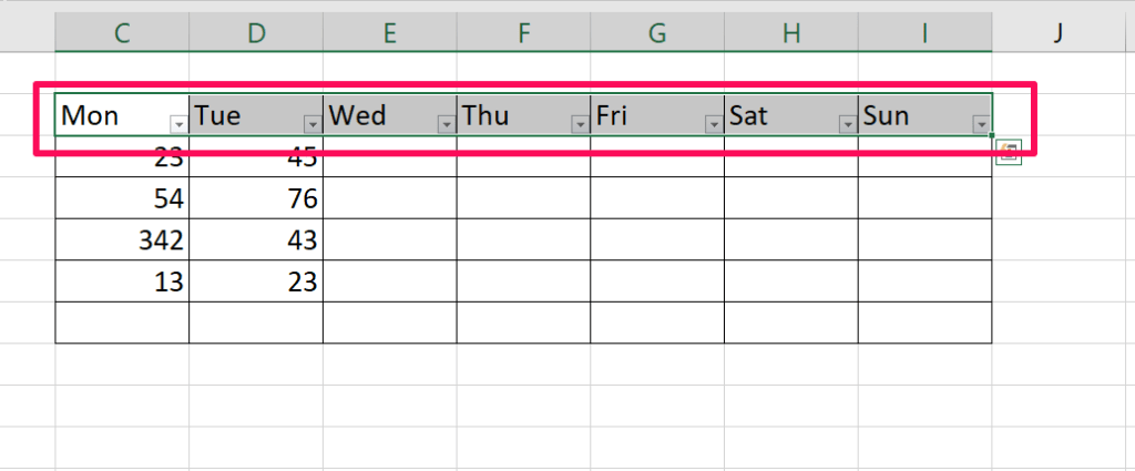
This shortcut comes in handy if you frequently filter different tables or data sets for information.

When you click on a filter, it gives you a dropdown of different options using which you can organize data in the filtered column.

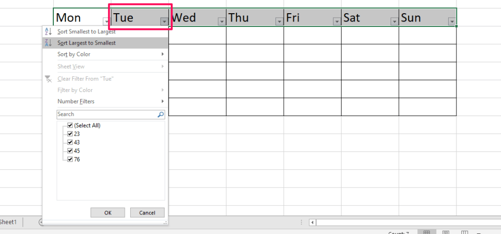
Plus, you can use the same shortcut to remove filters from a cell. Doing so will return the data set to its original unfiltered form.

Shortcut #3: Switch Between Cell Values And Formulas

This is a really useful keyboard shortcut for both advanced and new Excel users. It allows you to switch your view from cell values to formulas and vice versa.

To use it, just press CTRL + ~ anywhere in your worksheet. Let me explain this with a couple of screenshots.

Here’s the standard Excel sheet view in which the formulas are not visible.

And this is what you’ll see when you press CTRL + ~

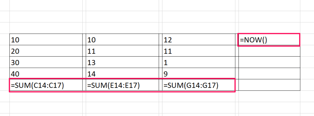
As you can see, all the formulas in the sheet are now visible to you.

This shortcut comes in handy if your Excel worksheet has different formulas and you want to frequently check how certain values are calculated.

Shortcuts #4: Add New Lines And Bullets In The Same Cell

This is one of my favorite Excel keyboard shortcuts.

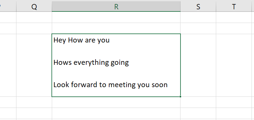
It allows you to enter long text descriptions and passages with multiple lines in the same cell.

It’s pretty simple.

Just double click on a cell to enter edit mode and press ALT + ENTER when you want to add a line in the same cell.

And that’s not all.

You can also add bullet points to this list using another shortcut: ALT + 7 (in the NUM keyboard)

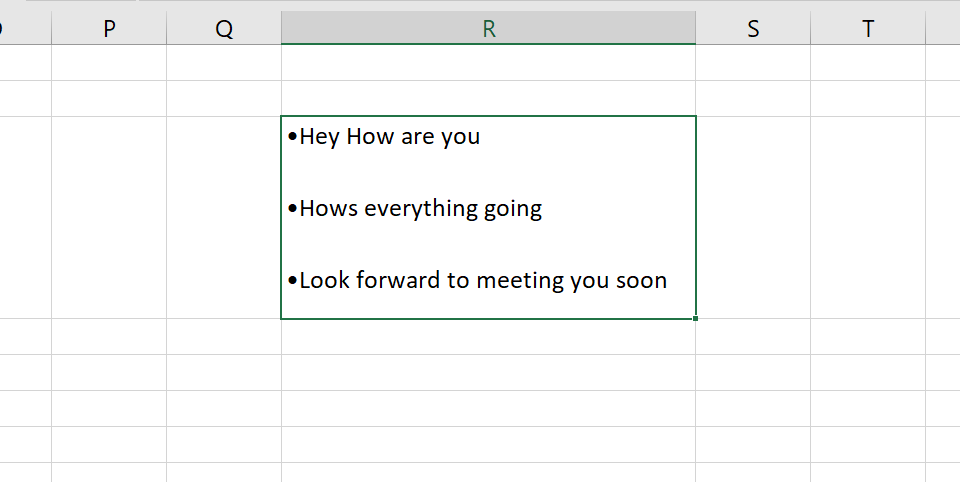
It’s a simple function but it helps you organize your content better without using extra cells or merging multiple cells to maintain alignment.

Shortcut #5: Insert The Current Date And Time In A Cell

If you don’t remember the current date or want to enter the exact time in a cell, use these handy keyboard shortcuts.

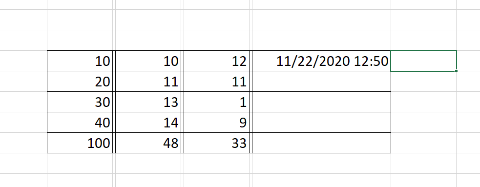
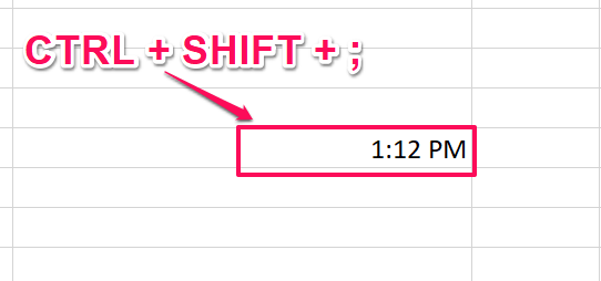
To enter the exact time, double click on a cell and press CTRL + SHIFT + ;

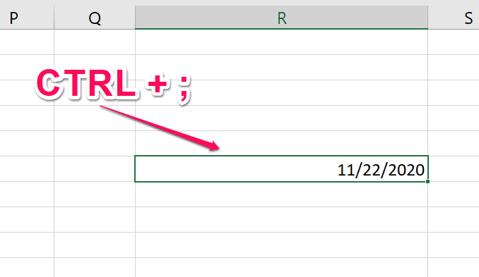
To get the current date, just press CTRL + ;

You can also enter both the values in the same cell by entering either the date or time first, then applying the other shortcut after hitting the space bar once.

MS Excel will display both the values in its default format; date as integers and time as decimal values.

Also, remember that the date and time in your selected cells will be entered as static text values. They’d only show the exact date or time when you used the shortcut. The values won’t be updated automatically when you open the document later.

To enter dynamic date and time values, you can use the NOW function in your Excel worksheets.

Shortcut #6: Insert The Sum Of Multiple Cells

It’s hard to imagine working in an Excel file and not using the SUM function to add different cell values.

It’s a pretty simple function but if you repeatedly use it by selecting all the cells you want to add, it can collectively take a big chunk of your time.

Why not use the easier way?

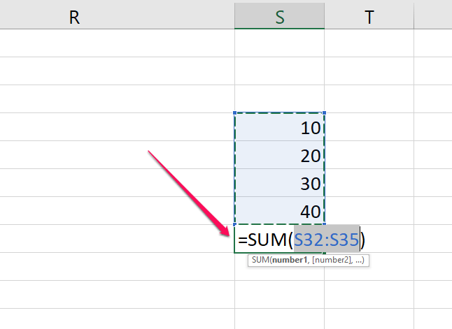
Just click on the cell right below the cells you want to add and press ALT + = to get the sum of all the cells above it without needing to select them first.

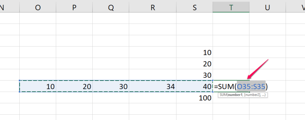
The same shortcut works if you want to get the sum of all the cells in a row.

Click on the cell just after the last cell of the row and press ALT + = to get the sum.

Using this shortcut will add the SUM function to your selected cell for all the preceding cells. You just need to press the ENTER key to apply it.

Shortcut #7: Create An Embedded Data Chart

I love using Microsoft Excel because of all the different charts and data visualizations it offers using which you can make your data look more engaging and easy to understand.

But adding charts can be time-consuming if you do it the regular way.

With this shortcut, however, you can instantly add a chart for any data set or table in a worksheet.

Here’s how it works.

Select the cells that you want to use in a chart

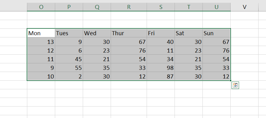
And then press ALT + F1 to create an embedded data chart.

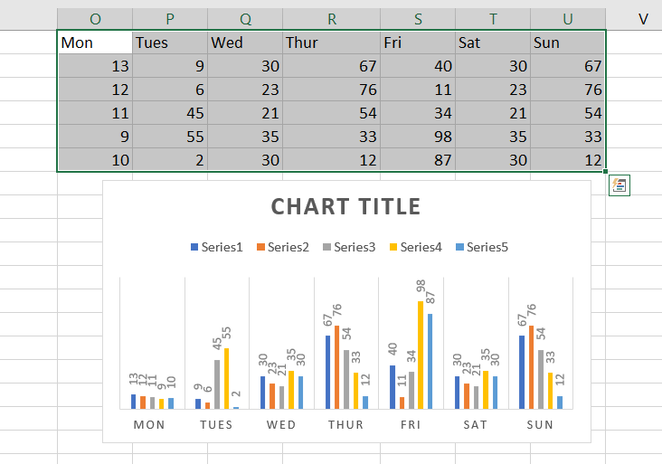
You can change the chart design by clicking any of the design options in the top menu.

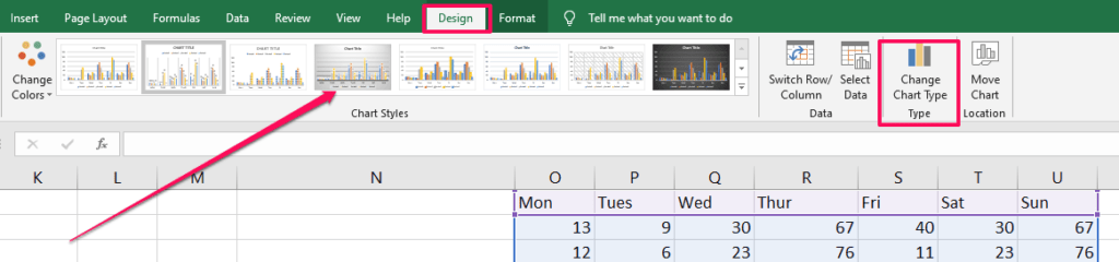
In case you want to use a different type of chart, you can choose it from the “Change Chart Type” section on the top menu.

Shortcut #8: Change Cell Color And Font Color

Colors play a vital role in making Excel sheets easy to understand and interpret.

If you’re like me and frequently use different colors in your worksheets, you’ll find this shortcut a big timesaver.

There are a couple of ways to change colors in Excel.

To fill color in one or more cells, select the cells and press ALT+H+H to open the color palette

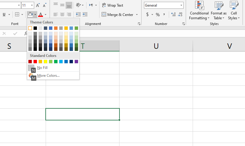
From here, choose the color that you want to fill in the selected cells.

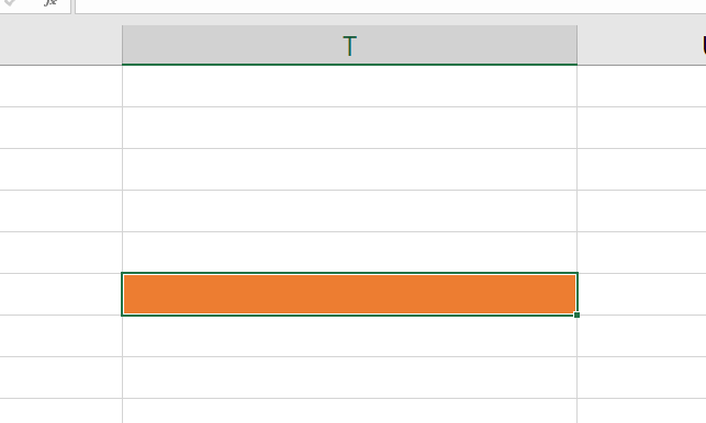
To change the font color, double click on a sell, select your desired text content, and press ALT+H+F+C to open the color palette.

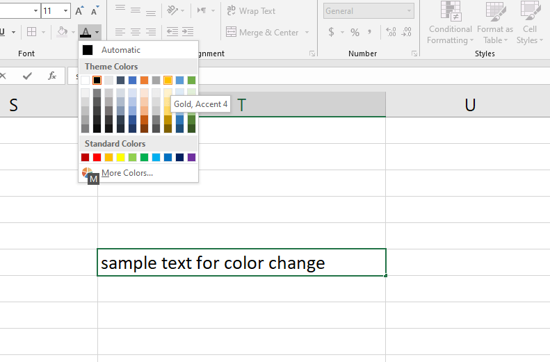
From here, choose any color you want.

For example, I selected the Gold color for only a part of the text in this screenshot.

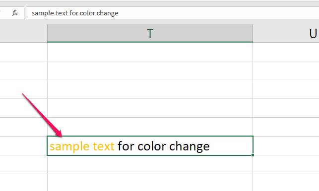
Using the right colors to highlight the key information in an Excel worksheet makes it much more user friendly. With these shortcuts, you’ll be able to colors much faster.

Shortcut #9: Apply Conditional Formatting

If you’re an advanced Excel user, you must be familiar with conditional formatting. But let me quickly explain it in case you haven’t heard of it.

Conditional formatting is a feature that allows you to apply specific formatting to the cells that meet certain criteria.

It is mostly used to highlight the cells with important information using different cell colors.

For example, you can use conditional formatting to turn any cell red where the value exceeds 1000 (or any other number).

This allows you to instantly identify the key information you need for decision making or to trigger any other action.

To apply conditional formatting, choose the cells where you want to use it and press ALT+O+D to open the Conditional Formatting Rules Manager.

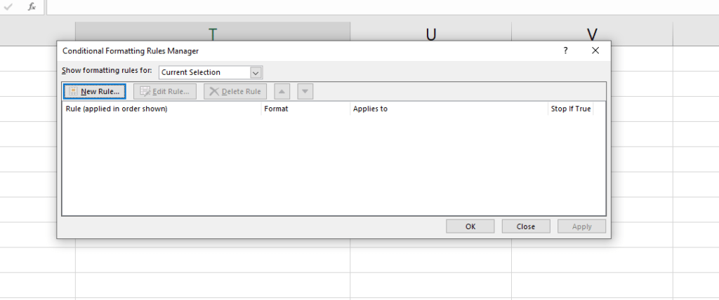
From here, you can set the rules to apply conditional formatting to different cells and the conditions to activate or deactivate it.

It’s a very useful feature for users handling large data sets out of which they have to identify different key values regularly.

For more details on how to use conditional formatting, and the tasks you can perform with it, read this article.

Shortcut #10: Use Paste Special For Multiple Options

Paste Special opens up a host of options to paste data in one or more cells in different ways.

But I’ll share just two keyboard shortcuts here that most users require on a day to day basis.

The first one allows you to copy the values from a cell without copying its format or formula.

For example, if the SUM formula is applied to a cell that shows the calculated value of 100, using Paste Special, you can copy the figure 100 to another cell without copying the cell’s formatting or its formula.

To use this option, copy the values from your desired cells and press ALT+H+V+V to paste them into another cell.

The other shortcut does the complete opposite.

It allows you to copy a cell’s formatting and formula and paste it into another cell without copying its actual value.

To use it, copy a cell’s formatting by pressing CTRL+C and then paste it to your desired cells by using ALT+E+S+T+ENTER

Shortcut #11: Use FlashFill

Flash Fill is a brilliant feature that can save you a ton of time if you’re doing repetitive work in MS Excel.

It detects data patterns in formatting based on your selection and replicates it in the cells you want.

You only need to provide the initial input based on which Flash Fill fills the remaining cells.

The keyboard shortcut for Flash Fill is CTRL+E.

Here’s how to use it.

Let’s say you have a database with student names and their roll numbers, like this.

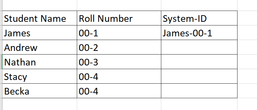
If you want Excel to automatically generate the System ID for all the students in the database, just give it the format of the first System ID as I’ve done in the screenshot above.

Then click on the cell below the first System ID entry and press CTRL+E to generate the remaining IDs with Flash Fill.

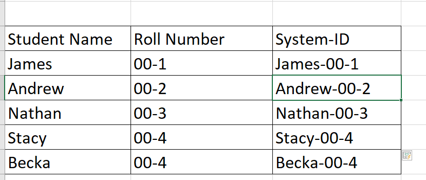
The Flash Fill column needs to be adjacent to the last column of your dataset (like in this screenshot).

You also need to provide the first entry in the Flash Fill column that Excel can use to generate the rest of the entries (like I entered James-00-1).

Using this shortcut, you can replicate formatting for thousands of cells in less than a second, saving you hours of work.

Shortcut #12: Freeze Rows And Columns

If you’re working with large data sets, you can easily confuse columns and repeatedly need to scroll to the top to ensure you’re entering data in the right cells.

You can get rid of this frustrating problem by using the Freeze Rows and Columns function.

Here’s how it works.

Simply select the top row of the worksheet that you want to freeze and press ALT+W+F+R.

Now you can scroll down all you want but the first row will stay in your view.

If you want to freeze a column, press ALT+W+F+C.